More About Excel Vlookup Example

Use VLOOKUP when you require to locate points in a table or an array by row. For instance, look up a rate of an automotive part by the component number, or discover an employee name based upon their employee ID. In its simplest type, the VLOOKUP feature claims: =VLOOKUP(What you want to seek out, where you want to try to find it, the column number in the range containing the worth to return, return an Approximate or Specific suit-- showed as 1/TRUE, or 0/FALSE).

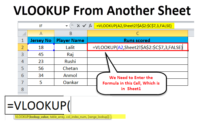
Utilize the VLOOKUP feature to look up a value in a table. Syntax VLOOKUP (lookup_value, table_array, col_index_num, [range_lookup] As an example: =VLOOKUP(A 2, A 10: C 20,2, TRUE) =VLOOKUP("Fontana", B 2: E 7,2, FALSE) =VLOOKUP(A 2,'Client Details'! A: F,3, FALSE) Disagreement name Description lookup_value (required) The worth you desire to look up. The worth you want to search for should remain in the first column of the variety of cells you specify in the table_array debate.

Lookup_value can be a worth or a recommendation to a cell. table_array (required) The variety of cells in which the VLOOKUP will search for the lookup_value and the return worth. You can use a called range or a table, and also you can make use of names in the argument as opposed to cell references.

The cell range additionally requires to consist of the return worth you wish to discover. Learn exactly how to choose ranges in a worksheet. col_index_num (called for) The column number (beginning with 1 for the left-most column of table_array) that includes the return worth. range_lookup (optional) A logical value that defines whether you desire VLOOKUP to locate an approximate or a precise suit: Approximate suit - 1/TRUE assumes the first column in the table is sorted either numerically or alphabetically, and will certainly then browse for the closest value.

For instance, =VLOOKUP(90, A 1: B 100,2, REAL). Exact suit - 0/FALSE look for the specific worth in the initial column. For instance, =VLOOKUP("Smith", A 1: B 100,2, FALSE). There are four pieces of info that you will need in order to build the VLOOKUP syntax: The worth you wish to look up, likewise called the lookup worth.

Excitement About Vlookup Example

Keep in mind that the lookup worth need to constantly be in the initial column in the array for VLOOKUP to work correctly. For instance, if your lookup value remains in cell C 2 after that your array ought to begin with C. The column number in the range which contains the return value. For instance, if you specify B 2:D 11 as the range, you ought to count B as the first column, C as the second, and also so on.

If you do not specify anything, the default value will always be REAL or approximate match. Currently place all of the above together as complies with: =VLOOKUP(lookup value, variety consisting of the lookup worth, the column number in the array including the return worth, Approximate suit (TRUE) or Exact suit (FALSE)). Here are a couple of examples of VLOOKUP: Problem What failed Incorrect value returned If range_lookup holds true or neglected, the first column requires to be sorted alphabetically or numerically.

Either sort the very first column, or make use of FALSE for a precise suit. #N/ A in cell If range_lookup holds true, after that if the value in the lookup_value is smaller than the tiniest value in the initial column of the table_array, you'll get the #N/ A mistake worth. If range_lookup is FALSE, the #N/ A mistake worth suggests that the precise number isn't located.

#REF! in cell If col_index_num is above the number of columns in table-array, you'll obtain the #REF! error value. To learn more on fixing #REF! errors in VLOOKUP, see Just how to correct a #REF! mistake. #VALUE! in cell If the table_array is less than 1, you'll get the #VALUE! mistake value.

#NAME? in cell The #NAME? error worth generally implies that the formula is missing out on quotes. To search for a person's name, make certain you make use of quotes around the name in the formula. For instance, enter the name as "Fontana" in =VLOOKUP("Fontana", B 2: E 7,2, FALSE). For additional information, see Just how to deal with a #NAME! mistake.

An Unbiased View of Vlookup

Discover just how to utilize absolute cell recommendations. Do not save number or day worths as text. When searching number or date worths, make certain the data in the very first column of table_array isn't saved as text worths. Otherwise, VLOOKUP could return a wrong or unforeseen worth. Arrange the initial column Sort the first column of the table_array prior to using VLOOKUP when range_lookup is REAL.

A concern mark matches any type of solitary personality. An asterisk matches any kind of series of characters. If you wish to find an actual enigma or asterisk, type a tilde (~) before the character. As an example, =VLOOKUP("Fontan?", B 2: E 7,2, FALSE) will certainly look for all circumstances of Fontana with a last letter that could differ.

When browsing text worths in the very first column, make certain the data in the initial column doesn't have leading spaces, trailing areas, inconsistent use straight (' or") and curly (' or ") quotation marks, or nonprinting personalities. In these cases, VLOOKUP could return an unforeseen value.

You can always ask a specialist in the Excel User Voice. Quick Recommendation Card: VLOOKUP refresher Quick Referral Card: VLOOKUP fixing tips You Tube: VLOOKUP video clips from Excel community specialists Every little thing you need to understand concerning VLOOKUP How to fix a #VALUE! error in the VLOOKUP function Just how to fix a #N/ A mistake in the VLOOKUP function Summary of formulas in Excel Exactly how to avoid busted formulas Detect mistakes in solutions Excel features (alphabetical) Excel features (by category) VLOOKUP (complimentary preview).

To determine shipping expense based upon weight, you can make use of the VLOOKUP feature. In the example shown, the formula in F 8 is: =VLOOKUP(F 7, B 6: C 10,2,1)* F 7 This formula utilizes the weight to locate the correct "expense per kg" then ... To override outcome from VLOOKUP, you can nest VLOOKUP in the IF function.

excel vlookup exact match excel vlookup not working text number excel vlookup between sheets